Exponential Smoothing
Contents
Introduction
When you select the Timeline chart “exponential” trend option, a trend line is fitted to the data. You can think of the line as similar to a moving average.
The underlying assumption is that the data varies around some intrinsic value that is fairly constant in the short term and changes gradually over time. Over the long term, this “average” value may trend up and down.
Exponential smoothing comes in three types:
- Simple – a moving average with higher weight to more recent data.
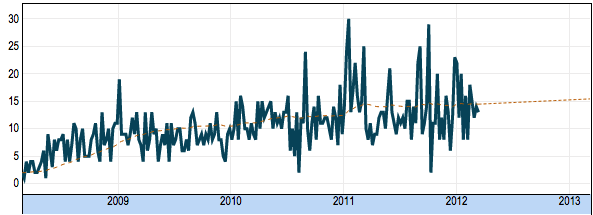
- Trend – in addition to calculating a moving average, we also calculate a moving estimate of the slope (up or down trend). The method produces a line that tracks the data more closely than simple smoothing and provides information for forecast.
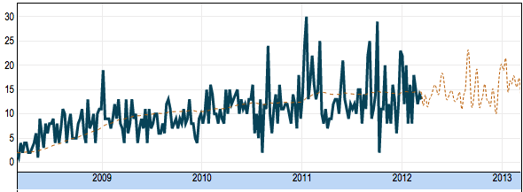
- Seasonality – in addition to calculating the trend line we just described, it also calculates weights for “multiplicative” seasonality. What we mean by “multiplicative” is, for example, that data for July tends to be 20% higher (multiple by 1.2) and data for February tends to be 10% lower (multiple by 0.9). Assuming that the data is indeed seasonal, we could use this information in the forecast part of the line.
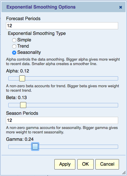
Exponential smoothing is very configurable and in the following sections we will describe the parameters, how they work and how best to set them.
Simple Smoothing
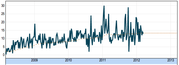
A simple exponential smoothing line can be thought of as a moving average that considers all the points behind the current point, but gives a somewhat higher weight to the more recent data.
The calculation is controlled by a parameter that’s referred to in the literature as “alpha”.
Alpha
This numeric value, between 0 and 1, controls the calculation. A smaller value (closer to 0) creates a smoother (slowly changing) line similar to a moving average with a large number of periods. A high value for alpha tracks the data more closely by giving more weight to recent data.
Considerations:
- Start with an alpha between 0.2 and 0.5 and see how it fits your data. Set it higher to fit changes in the data more closely. Set it lower to emphasize longer term trend.
- If you have lots of data points. For example, daily data for more than a year, then consider a lower alpha (even as low as 0.01 or 0.02) to include more of your timeline in the calculation.
Trend
This type of exponential smoothing also calculates an estimate of the slope. It tends to track the data more closely than simple smoothing, and is also useful for forecasting.
The calculation is controlled by both alpha and beta.
Beta
This numeric value, between 0 and 1, controls the trend calculation. A smaller value considers longer-term trend and a larger value focus on shorter-term trend.
Considerations:
- Start with a beta between 0.2 and 0.5 and see how it fits your data. Set it higher to reflect short-term trends.
- If you have lots of data points. For example, daily data for more than a year, then consider a lower beta (even as low as 0.01 or 0.02).
Seasonality
This option is useful for forecast if you assume seasonality in your data. The assumption is that data is cyclical and in each cycle, certain periods tend to be consistently higher or lower than the average.
This option assumes “multiplicative” seasonality where certain periods are higher or lower by a factor (for example 2 times or 0.4 times).
The term seasonality here refers to the entire cycle. For example, if you suspect that you have annual seasonality, then the cycle is one year.
The calculation of seasonality is based on two parameters: the length of the cycle (Season Periods) and a parameter referred to as “gamma”.
Season Periods
If the cycle is one year and the data is weekly, then the season period is 52 because there are 52 weeks in the cycle. Another example is if the “seasonality” is daily and the data is hourly, then set the Season Periods to 24 because the data cycles every 24 hours.
Gamma
Like with Alpha and Beta, this parameter is a numeric value between 0 and 1. A smaller gamma takes into account a longer history whereas a bigger gamma gives more weight to the recent history.
Conclusion
Let’s conclude with some suggestions for using this powerful feature effectively:
- Don’t always assume that the data has seasonality. If there’s no strong evidence for it, then it’s better not to use the seasonality feature.
- If you have less data than one cycle, for example if it’s an annual cycle and you have less than one-year worth of data, then you simply don’t have enough data for a forecast that accounts for seasonality and it’s best not use to use this feature.
- It’s okay to set beta to 0 if you suspect that the data doesn’t have any long-term trend.
- Consider whether recent changes in the data are a better predictor than the longer term trend. It’s often not obvious and your forecast is based on that assumption.


